
In production at last!
At last, at last, I think that the system is robust enough to be trusted with full runs without close monitoring. I still check the output for each dataset carefully, but things are going smoothly enough that I am now carrying out “production runs”, which I consider to be the final runs on the video data. I am currently working with camera AR50F, the best of the four, and things are going smoothly -- I expect to complete the data for this camera tonight. After that, it’ll be a matter of re-doing the data for the other three cameras. Then there’s the data from the FISTA aircraft: four more cameras with two hours of video apiece. Some of that video has not even been digitized yet; I shall begin work on that fairly soon, so that as one computer is preparing digital video for analysis, the second is carrying out that analysis. All of this will take a lot of time, but at this point it’s pretty much a matter of just running the programs and making sure that things don’t blow up. I’m guessing that the entire analysis will require another few weeks of work. In the meantime, I am spending most of my time on other projects; this project is now down to babysitting work.
I made a few changes in this final tweaking of the program. The biggest change was the new way to calculate the distance to the Leonid using its angular velocity. Initially, I had used the angular altitude of the Leonid to estimate its range, but there’s a big problem with that: the assumption that the linear altitude of the Leonid’s first appearance is always at 119 km. That number represents a good average for the Leonids we know, but it’s not reliable for this application. In the first place, small changes in the upper atmosphere can alter that number significantly. In the second place, we don’t know that the first flare that we see is actually the first instant that the Leonid hit the atmosphere -- a distant Leonid would be fainter and its first flares would not be visible at distance. But there is something that we know very accurately: the linear velocity of the Leonids as they hit the earth’s atmosphere. It’s 71.2 km/sec, and that number is highly reliable because it is derived from orbital calculations. If we know the linear velocity of a Leonid, and the geometry of its appearance, we can calculate its true range. However, calculating its apparent angular velocity purely from the geometry is not straightforward -- and I have to be able to predict that angular velocity correctly in order to identify Leonids. I had to use a bit of a kluge to deal with the predictive aspect of this. However, when analyzing Leonids that were actually observed, it’s much more straightforward: we know its angular velocity with pretty good accuracy (I’d guess about 2% accuracy). We also know the angle between the Leonid’s path and our line of sight: it’s equal to the distance between the Leonid and the radiant (think about it, and you’ll figure it out). This means that we can use the angular velocity and the linear velocity to calculate the range with some accuracy.
This led to another change: I have previously been calculate the longitude, latitude, and height of each Leonid. That’s actually nonsensical: the Leonid traverses a lot of space and so it’s meaningless to talk about its position. Instead, we need to think in terms of the positions of each of the flares. I have therefore changed the data report to assign latitude, longitude, and height to each individual flare rather than the Leonid as a whole.
It has been fascinating to audit the Leonid reports. I go through them, comparing previous reports with the latest report, looking for differences. I’m finding that the newest algorithms typically find about 2% more Leonids than the previous algorithms, and the Leonids they are catching are truly tiny. It really is amazing how good those algorithms are at nailing the tiniest Leonid without also reporting false positives. Indeed, the newest algorithms are even better at rejecting false positives than the earlier algorithms. I know that they’re not perfect: I’m certain that some Leonids are missed and that there are a few false positives in the reports. But I estimate that these errors apply to well under 1% of all the Leonids in the reports.
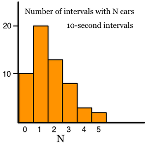
Once all the data is accumulated, I’ll start work on the actual science. There are a bunch of tests that I want to run. Dr. Jenniskens has his own interests, and I shall probably take some time catering to his requests, but most of the data I can transmit to him directly for his own analysis. But my first test will be a quick test for temporal non-randomness. This subject has been studied extensively and all the papers so far have found no evidence of temporal non-randomness. However, I believe that there is temporal non-randomness at time scales of a few seconds. This is an important concept: non-randomness is dependent upon the time scale you use. Think of it this way: Suppose that you’re wondering whether the traffic passing your house, which sits on a large boulevard, is random. So you carry out a simple statistical test. You count all the cars that pass your house for ten seconds, then write down that number. Then you count all the cars in the next ten seconds, and the next ten seconds, and so on for several hours. Then you plot a histogram of how many times you counted no cars, how many times you counted one car, two cars, three cars, and so on. Suppose that the histogram looks like this:
Here’s what your histogram would look like if the cars were perfectly random:
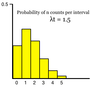
As you can see, your data closely match the theoretical distribution and so strongly support the belief that the cars came randomly. However, the fact that they come randomly in 10-second intervals doesn’t mean that they are totally, completely random. Suppose that, just half a mile up the boulevard there’s a traffic light with a cycle time of 96 seconds. That is, it goes through a complete cycle every 96 seconds. Suppose also that you were to repeat the experiment above, except that you used 48-second intervals instead of 10-second intervals. Then your intervals will split the 96-second cycle of the traffic light exactly in half; one 48-second interval will see a bunch of cars that went through the green light, and the next 48-second interval won’t have many cars, reflecting the red light. If you do this for an hour or two, about half of your intervals will show lots of cars, and the other half will show few cars, like this:
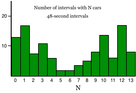
This isn’t random at all! As you can see, the interval size you select determines a great deal about what kind of non-randomness you find. Now, this is a contrived example, and it’s not directly applicable to the problem of non-randomness of shower meteors, because there aren’t any traffic lights in space. But it does serve to demonstrate that what kind of randomness you observe depends upon the interval size. In other words, a proper analysis should examine a range of interval sizes. For my Leonid analysis, I intend to examine interval sizes from 1 second to 20 seconds.
But there’s another problem. The formula for the Poisson distribution, which is what we use for this kind of situation, looks like this:

Here, P(n) is probability of seeing n events in an interval t seconds long, with an average rate of λ events per second. This assumes that the events (in this case, appearances of Leonids) are coming at a constant rate. But that isn’t the case with our Leonids; the rate rose steeply from 1:00 AM to 2:05 AM, peaked at 2:05 AM, then fell rapidly. So how can I compare periods of time when the rate was changing? Typically you handle problems like this by integrating (as in calculus) the probability function over the period in question. Unfortunately, this tends to smear out the distribution, making it even more difficult to detect any non-randomness. I have therefore decided upon a different approach: a distribution of distributions. Here’s the idea:
I separate the time series of Leonid events into one-minute segments. For each one-minute segment, I use the standard Poisson equation, using a constant value for λ for that minute. This gives me two distributions: the observed distribution of Leonid events and the predicted distribution. This might look like this:
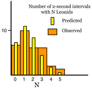
Now all we do is carry out a standard χ² test on these two distributions. (I’m sorry, I won’t explain the χ² test here.) This will give us a number for the non-randomness of the observed distribution -- technically, the probability that the observed distribution would have been produced by a random process. I’ll carry out this process for each of the minutes in, say, the one-hour period centered on the moment of maximum rate. This gives me 60 Poisson distributions and 60 χ² results. I then put those χ² values into another distribution, and the end result had better look like the standard χ² distribution. The degree to which it deviates from the standard χ² distribution is the measure of the non-randomness of the Leonids. Remember, I have to carry out this procedure for many different time intervals: 1-second, 2-second, 3-second, etc.
And that’s all there is to it!